Beyond Labels: The Magic of Autoencoders in Unsupervised Learning
- shivamshinde92722
- Oct 10, 2024
- 6 min read
In a world where labeled data is often scarce, autoencoders provide a powerful solution for extracting insights from unstructured data

Agenda
Unlabeled Data
Auto-Encoders: Loss Function, Bottleneck, Denoising Auto-Encoder
Unsupervised Pre-training Using Auto-Encoders
Code Demonstration
Unlabeled Data
In many applications, such as object recognition and detection, collecting labeled data is challenging, while unlabelled data is relatively easy to gather. We can leverage this abundant unlabelled data to enhance the performance of our models.
A useful approach is to use the unlabeled data to learn meaningful representations of the input features. In image-related tasks, for example, the early layers of a neural network typically learn basic abstract features of an image, such as edges and other basic shapes. By using a large amount of unlabeled data, we can train the network to extract these foundational features. Once these abstract representations are learned, we can then train the new neural network, with the abstract features serving as inputs. This approach generally leads to improved model performance.
A type of neural network called ‘Autoencoder’ is used to calculate this representation.
Auto-Encoders
Here,
Let X1, X2, …, Xm represent the inputs to the auto-encoder neural network, h1, h2, …, hk represent the condensed or essential features of the input, and the reconstructed outputs are denoted by X1′,X2′,…,Xm.
In this network, we feed image pixels as input. The middle hidden layer captures the condensed essence or representation of the input features. The goal is to then reconstruct the original input from this condensed representation.
The first part of the network, where the input is transformed into its essential features, is known as the encoder. The second part, where the essence is used to reconstruct the original input, is called the decoder.
For auto-encoder neural networks, the number of neurons in hidden layers first decrease during encoder part and then increase during decoder part of the network.
Note that, in the figure I have shown only one hidden layer. However, we can have multiple hidden layers in encoder and decoder part of the network. Also, we can have different number of hidden layers in the encoder and decoder part of the neural network.
Auto-encoder training loss function
With auto-encoder, our main goal is to create the values of outputs (reconstructed inputs) as close as possible to inputs. We can use Mean Squared Error as a performance measure.
This loss is called reconstruction loss. So, in short, our goal is to minimize this reconstruction loss.
Note that reconstruction loss function does not require any training labels.
Bottleneck
If number of neurons in input (m) is equal to number of neurons in hidden layer (k), then consider the case where activation function is linear, W1 = W2 = I (identity matrix) and b1 = b2 = 0.
In this case input and reconstructed values will be equal but model won’t learn proper essence of input in the hidden layer.
For this reason, we generally set k < m. Therefore, hidden layer is called bottleneck.
Denoising AutoEncoder
However, there is a way we can use k ≥ m.
If we first add some noise to the inputs and then use the auto-encoder to reconstruct the original inputs without noise, then we can use k ≥ m. Even if the activation is linear and W1 = W2 = I (identity matrix), b1 = b2 = 0, then also we won’t get zero reconstruction error.
We are adding the noise N(0, I) to the input and we will try to reconstruct the input X using the autoencoder.
Unsupervised Pre-training using Auto-Encoder
After training the autoencoder, W1 and b1 learn to extract the useful features from the input. Now we can use these extracted features for different tasks such as image classfication.
Usually, extracted feature from the hidden layer is of smaller dimension than input. So, this works kind of like dimensionality reduction.
Also, if we used the extracted features for classification then we might get the better performance than normal classfication in most cases. This is because, the encoder is trained on much larger unlabelled dataset. So, it learns the abstract features of the image better than when we use the smaller dataset for the classfication task.
We ‘chop-off’ the decoder part of auto-encoder and then add new layers after the encoder part to create a new neural network for the classfication.
During the training of classification model, we only train the neurons in the secondary network. But we can fine-tune the trained auto-encoder with small learning rate or we can even make the encoder layers untrainable.
Now, let’s see how to use auto-encoders for unsupervised pretraining using the code.
Code Demonstration
We will be using MNIST Fashion dataset for out task.
Importing required libraries and preprocessing the data
# Importing required libraries

import warnings
warnings.filterwarnings('ignore')

import numpy as np
import tensorflow as tf
import tensorflow as tf
from tensorflow.keras.models import Model
from tensorflow.keras.layers import Input, Dense
from tensorflow.keras.callbacks import EarlyStopping
from sklearn.metrics import accuracy_score

# Loading the MNIST dataset
mnist = tf.keras.datasets.mnist
(x_train, y_train), (x_test, y_test) = mnist.load_data()

# Normalizing the data by scaling pixel values from [0, 255] to [0, 1]
x_train, x_test = x_train / 255.0, x_test / 255.0

# Reshaping the data:
x_train = x_train.reshape(-1, 784)
x_test = x_test.reshape(-1, 784)
Training the encoder network
# Creating an autoencoder model
# Input layer: expects a 784-dimensional vector (flattened image)
ip = tf.keras.layers.Input(shape=(784,), name='input')

# Encoder layers
x = tf.keras.layers.Dense(512, activation='relu', name='encoder1')(ip)
x = tf.keras.layers.Dense(256, activation='relu', name='encoder2')(x)
x = tf.keras.layers.Dense(128, activation='relu', name='encoder3')(x)

# Essence layer
essence = tf.keras.layers.Dense(64, activation='relu', name='essence')(x)

# Decoder layers
x = tf.keras.layers.Dense(128, activation='relu', name='decoder1')(x)
x = tf.keras.layers.Dense(256, activation='relu', name='decoder2')(x)
x = tf.keras.layers.Dense(512, activation='relu', name='decoder3')(x)

# Output layer
op = tf.keras.layers.Dense(784, activation='relu', name='reconstructed_input')(x)

# Define the autoencoder model
# - inputs=ip: input layer
# - outputs=op: output layer (reconstructed input)
model = Model(inputs=ip, outputs=op)

# Compile the model
model.compile(optimizer='adam', loss='mse', metrics=['accuracy'])

# Display the summary of the model architecture
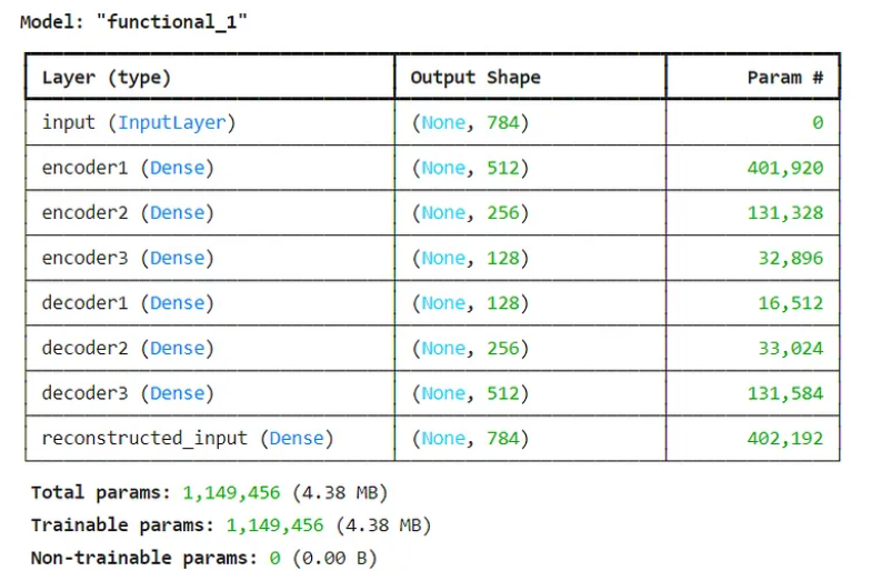
model.summary()

# Define early stopping to prevent overfitting
early_stopping = EarlyStopping(monitor='val_loss', min_delta=0, patience=10, verbose=1, mode='auto')

# Train the model using the autoencoder framework
history = model.fit(x_train, x_train,  # input and output should both be the training data for autoencoders
                    epochs=20,
                    batch_size=2048,
                    validation_data=(x_test, x_test),
                    callbacks=[early_stopping])
Getting the essence layer of the encoder for later classification tasks
# Define the encoder model
encoder = Model(inputs=ip, outputs=essence)
Training the classfication model without using auto-encoder’s extracted features
# Define the neural network model
ip = tf.keras.layers.Input(shape=(784,), name='input')
x = tf.keras.layers.Dense(128, activation='relu')(ip)
x = tf.keras.layers.Dense(64, activation='relu')(x)
output = tf.keras.layers.Dense(10, activation='softmax')(x)

# Create the model that connects the input layer to the output layer
normal_model = Model(inputs=ip, outputs=output)

print("Normal Model Summary:\n")
print(normal_model.summary())

# Compile the model
loss='sparse_categorical_crossentropy', metrics=['accuracy'])

# Early stopping to prevent overfitting:
early_stopping = EarlyStopping(monitor='val_loss', min_delta=0, patience=10, verbose=1, mode='auto')

# Train the model:
normal_model.fit(x_train, y_train,
                 epochs=20,
                 batch_size=2048,
                 validation_data=(x_test, y_test),
                 callbacks=[early_stopping])

# Make predictions on the test data:
y_hat_prob = normal_model.predict(x_test)

# Convert the predicted probabilities to class predictions:
y_hat = np.argmax(y_hat_prob, axis=1)

# Calculate accuracy:
acc = accuracy_score(y_test, y_hat)

# Print the accuracy of the model on the test set
print(f'Accuracy: {acc}')
Note that we are getting approximately 97.38% accuracy over the testing data when we don’t use the auto-encoder’s extracted features.
Training the classfication model using auto-encoder’s extracted features (Unsupervised Pretraining)
# Freeze the encoder layers to prevent them from being updated during training (Optional)
for layer in encoder.layers:
    layer.trainable = True # Not freezing layers

# Define the model that will be trained on the encoded data
ip = tf.keras.layers.Input(shape=(784,), name='input')
x = encoder(ip)
x = tf.keras.layers.Dense(128, activation='relu')(x)
x = tf.keras.layers.Dense(64, activation='relu')(x)
output = tf.keras.layers.Dense(10, activation='softmax')(x)

# Create the model that includes the frozen encoder and new classification layers
pretrained_model = Model(inputs=ip, outputs=output)

print("Normal Model Summary:\n")
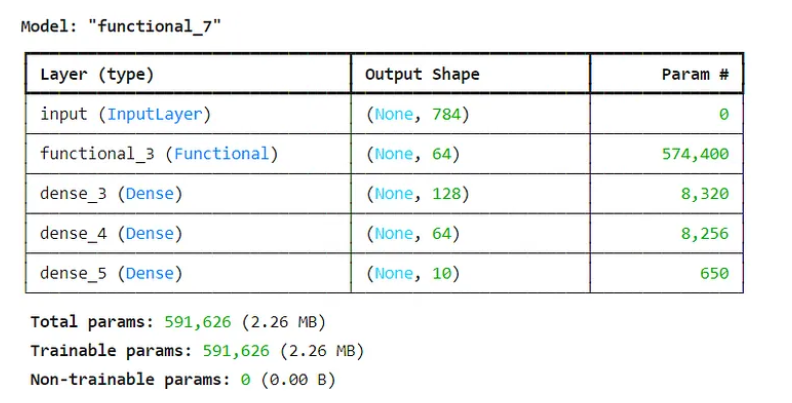
print(pretrained_model.summary())

# Compile the model using Adam optimizer and sparse categorical crossentropy loss (for integer labels)
pretrained_model.compile(optimizer='adam', loss='sparse_categorical_crossentropy', metrics=['accuracy'])

# Early stopping to prevent overfitting; stops if validation loss doesn't improve for 10 epochs
early_stopping = EarlyStopping(monitor='val_loss', min_delta=0, patience=10, verbose=1, mode='auto')

# Fit the model on training data (x_train) with validation on x_test
pretrained_model.fit(x_train, y_train,
                     epochs=20,
                     batch_size=2048,
                     validation_data=(x_test, y_test),
                     callbacks=[early_stopping])

# Predict the class probabilities on the test set
probs = pretrained_model.predict(x_test)

# Convert probabilities to class predictions using argmax (highest probability wins)
y_hat = np.argmax(probs, axis=1)

# Calculate accuracy by comparing predictions (y_hat) to actual labels (y_test)
acc = accuracy_score(y_test, y_hat)
print(f'Accuracy: {acc}')
Note that we are getting approximately 97.84% accuracy over the testing data when we use the auto-encoder’s extracted features. This is better accuracy as compared to when we don’t use auto-encoder’s extracted features.
Also, note that I have made the encoder’s layers trainable in this case. But we can also freeze encoder’s layers and only train the secondary network. Optionally, we can also train the encoder using very learning rate.
Thank you so much reading. Have a great day!


Comments