From Many to Few: Tackling High-Dimensional Data with Dimensionality Reduction in Machine Learning
- shivamshinde92722
- Jul 2, 2023
- 4 min read

This article will discuss the curse of dimensionality in machine learning problems and dimensionality reduction as a solution for the issue.
What is the Curse of Dimensionality? Sometimes a machine learning problem may consist of thousands or even millions of features for every training instance. Training our machine learning model on such data is extremely resource-consuming as well as time-consuming. This problem is often regarded as the ‘Curse of Dimensionality’.
Resolving the issue of high-dimensionality To tackle the curse of dimensionality, we often employ different methods that reduce the number of features (in other words, the number of dimensions) in the data.
The Usefulness of Dimensionality Reduction Methods Dimensionality reduction methods help in preserving resources as well as time. In rare cases, the reduction may even help filter out the unnecessary noise from the data. Another use of dimensionality reduction is the visualization of data. Since the visualization of high-dimensional data is hard to perform and also hard to understand even if we succeed to visualize it, reducing the dimension to 2 or 3 often helps us visualize the data more clearly.
Demerits of reducing the dimensionality of the data The dimensionality reduction methods are not without demerits. Loss of information occurs when we perform dimensionality reduction on the data. Also using the dimensionality reduction method on the data does not guarantee the increase in the performance of the model. Note that these methods are just a way to train the model faster or preserve our resources but not a way to increase the performance of the model. In most cases, the performance of the model trained on the reduced data will be poor in comparison with the model which is trained on the original data.
There are two famous approaches to the dimensionality reduction.
Projection
Manifold Learning
Projection In most real-world problems, the features of the data are not equally spread across all dimensions. Some are almost constant and others are correlated. Therefore, these training instances lie within or quite close to the much lower sub-space of the original high-dimensional space. In other words, there exists a lower dimensional representation of the data that is almost equivalent to the representation of data in its original space.
But this approach is not the best approach for all types of datasets. For some datasets, using the projection method will squash the different layers of instances together and such projection won’t represent the original data into the lower dimensions. For this type of data, manifold learning methods are more suitable.
Manifold Learning In the manifold learning method, we unroll the data rather than projecting it onto the lower subspace.
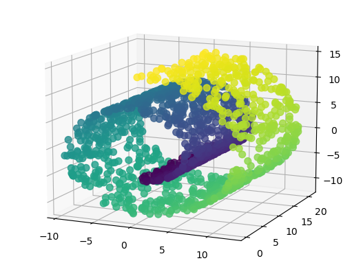
Let’s consider an example of the Swiss Roll dataset to understand manifold learning. As shown in the visualization of the Swiss Roll dataset above, one cannot find the projection of the data without overlapping many data instances onto each other. So in this kind of case, rather than projecting onto the lower subspace, we unroll this data. This means we will unroll the data points shown above in a 2D place and then make sense of it.
Now let’s understand one of the most popular and widely used dimensionality reduction methods known as Principal Component Analysis (PCA).
PCA is the projection kind of method. It first finds the hyperplane that is closer to it and then projects the data onto it.
There are two ways of finding the right hyperplane for projection:
Finding the hyperplane that preserves the maximum amount of variance of the original dataset after projecting it onto the hyperplane.
Finding the hyperplane that gives the lowest value of the mean squared distance between the original dataset and its projection onto the hyperplane.
Note that we use variance as a measure because the variance of the dataset represents the amount of information it contains.
PCA finds the axes (i.e. principal components) of the hyperplane that account for the largest amount of variance.
Let’s understand the way one can perform this. For the demonstration of PCA, we will use the wine-quality dataset.
Method 1
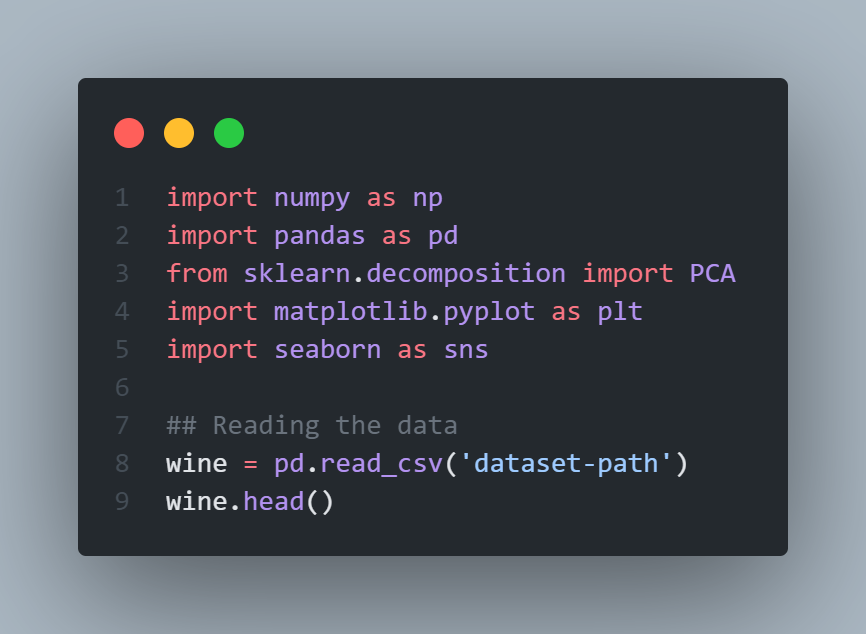
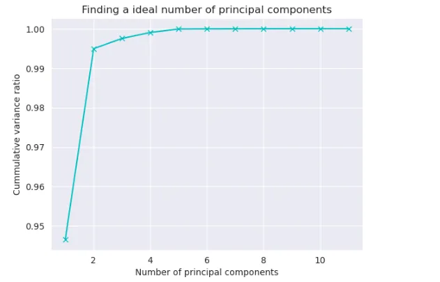
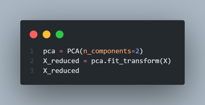
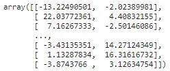
In this method, we will train the PCA class with its default settings and then find out the variance contributed by each of the principal components. Then we will find out the number of principal components which give the highest amount of variance upon addition. Then use this ideal number of principal components to train the PCA class again.


Decompressing the data
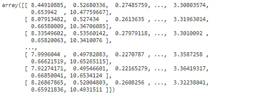
It is also possible to decompress the data into its original size using inverse_transform function. Obviously, this won’t give us the original dataset as it is since we have lost a part of the information (about 5%) in the reduction process. But still, this decompressing will give us the dataset which is quite close to the original dataset.

There are many variants of the PCA algorithm: Randomized PCA, Incremental PCA, Kernel PCA, etc.
Also besides this popular PCA algorithm, there are many other dimensionality reduction algorithms such as isomap, t-distributed stochastic neighbor embedding (t-SNE), linear discriminant analysis (LDA), etc.
I hope you like the article. If you have any thoughts on the article then please let me know. Any constructive feedback is highly appreciated.
Have a great day!


Comments