From Vanilla RNNs to LSTMs: A Practical Guide to Long Short-Term Memory
- shivamshinde92722
- Jan 6, 2023
- 3 min read
Long short-term memory (LSTM) networks have become a go-to tool for tasks like machine translation, language modeling, and speech recognition. But what exactly are LSTMs, and how do they work? In this post, we’ll provide a high-level overview of LSTM’s working.

Due to the transformation that the data goes through when going through the RNN network, some information is forgotten at each time step. And, if the sequence is long enough then by the time data reaches the last time step, it won’t remember anything from the beginning of the sequence.
Different types of long-term memories have been introduced over the year to amend this problem. Long short-term memory aka LSTM is one of them.
Let’s understand how LSTM works!
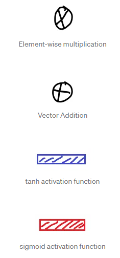
Meaning of symbols in diagrams
Note the meaning of the symbols in the below diagrams:

Meaning of variables in the equations
Wxi, Wxf, Wxo, Wxg are the weight matrices of each of the four gates for their connection to the input vector x(t).
Whi, Whf, Who, Whg are the weight matrices of each of the four gates for their connection to the previous short-term state h(t-1).
bi, bf, bo, bg are the bias terms for each of the four gates.
Basic info about the LSTM cell
On a high level, one can consider LSTM as a cell that is similar to the basic recurrent neural network (RNN) cell but with a long memory.
Unlike the basic RNN cell, the state of the LSTM is divided into two parts. One is responsible for the long-term memory of the network and the other is responsible for the short-term memory of the network.
The LSTM cell is made of four blocks. They are
Basic RNN block, g(t)
forget gate, f(t)
input gate, i(t)
output gate, o(t)
Also, the LSTM cell takes in three inputs. They are
Previous cell’s long-term state, c(t-1)
Previous cell’s short-term state, h(t-1)
Training data input, x(t)
The LSTM cell outputs three terms. They are
Current cell’s long-term state, c(t)
Current cell’s short-term state, h(t)
Predictions for the current cell, y(t)
Now, let’s understand how each of the outputs is calculated given the inputs from the previous cell.
Calculating the long-term state of the current cell
The long-term state is calculated using the two parts of the LSTM’s internal networks. One consists of the forget gate and the other consists of the input gate and basic RNN cell.

This is the first part used to find long-term memory. The purpose of the first part is to know what should be forgotten from the past. Previous short-term state h(t-1) and the training data input x(t) are multiplied by their respective weight vectors and then the bias vector is added to their sum. This whole sum is used as input to the sigmoid activation function. This restricts the value of f(t) between 0 and 1.

The output f(t) of the forget gate is multiplied by the previous cell’s long-term state. Basically, the purpose of the forget gate is to know how much to forget from the previous long-term state. The green-colored part in the above figure represents the value after forgetting something from the past.

The purpose of the second part is to know what should be retained from the new inputs. The input gate is a kind of controller that determines how much of the output of the basic RNN cell should be retained in the present time step. The retained output is the second part which is added to make the current long-term memory. The retained output of the basic RNN cell is represented by the 2 in green color in the above figure. The equations are similar to part 1.


The value of the current long-term state is represented in the above diagram using the addition of ‘1’ and ‘2’ in green color.
Calculating the short-term state and the predictions of the current cell

Basically, the predictions and the short-term state have equal value. So, if we find any one of the values then another is found as well. Let’s find the short-term state.
The short-term state is calculated using the two parts. The first part is the output of the output gate. Another part is found by applying the hyperbolic tangent activation function to the current long-term state.
We get the value of the short-term state after the multiplication of part 1 and part 2.

Until now we have seen the different parts of the whole LSTM to understand it better. So, let’s combine all of the above parts to create a whole diagram of the LSTM cell.

This is the whole LSTM network.
I hope you like the article. If you have any thoughts on the article then please let me know.
Have a great day!


Comments